simulations

Plancherel growth of Young diagrams

Plancherel growth of Young diagrams

Plancherel measures

Let $G$ be a finite group and $\widehat G$ the set of all (equivalence classes of) irreducible representations of $G$. For any $\lambda\in \widehat G$ we denote by $d_\lambda$ the dimension of the associated irreducible representation. In the representation theory, it is well known that $|G|=\sum_{\lambda\in \widehat G}d_\lambda^2.$ Therefore, we obtain a probability measure $\mathbb{P}\mathrm{Pl}$ on $\widehat G$ by $\mathbb{P}_\mathrm{Pl}(\lambda):=\frac{d_\lambda^2}{|G|} \quad (\lambda \in \widehat G).$ This probability measure $\mathbb{P}\mathrm{Pl}$ is called the Plancherel measure of $G$.

Young diagrams and Symmetric groups

Young diagrams

A Young diagram is a non-increasing sequence $\lambda=(\lambda_1\geq \lambda_2\geq \cdots)$ of nonnegative integers such that $|\lambda|:=\sum_{i=1}^\infty\lambda_i<\infty$. We call $|\lambda|$ the size of $\lambda$. By definition, there exists an integer $l(\lambda)\geq 0$, called the length of $\lambda$, such that $\lambda_{l(\lambda)}\neq 0$ and $\lambda_{l(\lambda)+1}=0$.

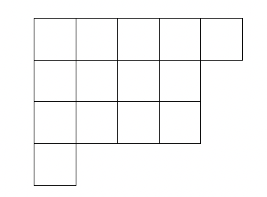
Let $\mathbb{Y}_N$ denote the set of Young diagrams with size $N$. Usually, a Young diagram $\lambda\in \mathbb{Y}_N$ is represented as a diagram, which consists of $N$ boxes arranged in left-justified rows. The number of boxes in each rows is $\lambda_1, \lambda_2, \dots$ from top to bottom. For instance, $\lambda=(5, 4, 4, 1)$ is represented by the following diagram:

result

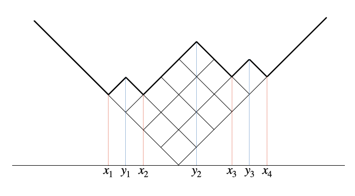
In analysis, the following rotated (and reflected) display is also useful:

result

We assume that the edge length of each box is $\sqrt{2}$. The bold line is called the profile of a Young diagram $\lambda$. We denote by $x_1, x_2, \dots, x_r$ and $y_1, y_2, \dots, y_{r-1}$ the local minima and local maxima of the profile, respectively. By assumption, they are integers. Moreover, the following interlacing inequalities holds: $x_1<y_1<x_2<\cdots <y_{r-1}<x_r.$ We call them the min-max coordinate of $\lambda$. We remark that Young diagrams are implemented as those min-max coordinates in the coding below. The following characterization of min-max coordinates is known: An interlacing integers $x_1<y_1<x_2<\cdots <y_{r-1}<x_r$ is the min-max coordinate of some Young diagram if and only if $\sum_{i=1}^rx_i-\sum_{i=1}^{r-1}y_i=0$ holds.

Symmetric groups

Let $S(N)$ denote the symmetric group of degree $N$. In the representation theory, it is well known that $\widehat{S(N)}$ is parametrized by $\mathbb{Y}_N$. Thus, the Plancherel measure of $S(N)$ is identified with a probability measure on $\mathbb{Y}_N$.

Let us mention an explicit formula of the Plancherel measure of $S(N)$. We remark that this formula is not used in the coding below. Instead of this, we realize the Plancherel measure of $S(N)$ by the interval shrinkage algorithm suggested by S. V. Kerov.

For any Young diagram $\lambda$ we denote by $\lambda’$ its transpose, that is, $\lambda’$ is obtained by replacing columns and rows of $\lambda$. More precisely, we have $\lambda'_i=|\{j\geq 0\mid \lambda_j\geq i\}|\quad (i=1, 2, \dots)$

We denote by $d_\lambda$ the dimension of the irreducible representation of $S(N)$ labeled by $\lambda\in \mathbb{Y}N$. The following hook-lenght formula is well known: $d_\lambda = \frac{N!}{\prod_{i=1}^{l(\lambda)}\prod_{j=1}^{\lambda_i}(\lambda_i-i+\lambda'_j-j+1)}.$ Since $|S(N)|=N!$, we obtain the following explicit formula of the Plancherel measure $\mathbb{P}\mathrm{Pl}$ of $S(N)$: $\mathbb{P}_\mathrm{Pl}(\lambda) = \frac{N!}{\prod_{i=1}^{l(\lambda)}\prod_{j=1}^{\lambda_i}(\lambda_i-i+\lambda'_j-j+1)^2} \quad (\lambda\in \mathbb{Y}_N).$

Plancherel growth of Young diagrams

For $\lambda\in\mathbb{Y}N$ and $\nu\in\mathbb{Y}{N+1}$, we write $\lambda\nearrow \nu$ when $\nu$ is obtained by adding one box to $\lambda$. We consider a growth process of Young diagrams $\lambda^{(1)}\nearrow \lambda^{(2)}\nearrow\cdots.$ If this growth occurs randomly and $\lambda^{(N)}$ is distributed by the Plancherel measure of $S(N)$ for each $N\geq1$, we call this growth a Plancherel growth.

In the actual coding, we will realize a Plancherel growth by the interval shrinkage algorithm suggested by S. V. Kerov. Let us explain this here. First, we assume that $\lambda$ is a current Young diagram. Let $x_1<y_1<x_2<\cdots <y_{r-1}<x_r$ denote the min-max coordinate of $\lambda$. To obtain a new Young diagram, we should choose one of the local minima $x_1, \dots, x_r$ and add one box to this point. By the interval shrinkage algorithm, we will determine one of the local minima $x_1, \dots, x_r$. We first have the interval $[x_1, x_r]$ and take $X_1$ uniformly distributed in $[x_1, x_r]$. Then, we shrink our interval $[x_1, x_r]$ by the following rule. If $x_i<X<y_i$, then the next shrank interval is $[x_1, x_i]$. If $y_i<X<x_{i+1}$, then the next shank interval is $[x_{i+1}, x_r]$. In the next step, we apply the same shrinkage procedure for the resulting interval. We continue these steps until the interval shrinks to one point. Moreover, the resulting point is a point we seek to add a box.

Limit shape

Let $(\lambda^{(N)}){N\geq1}$ be a Plancherel growth sequence of Young diagrams. For each $N\geq 1$ we denote by $\omega{\lambda^{(N)}}$ the profile of $\lambda^{(N)}$. Namely, $\omega_{\lambda^{(N)}}$ is a piecewise linear function on $\mathbb{R}$ such that its slope is $\pm 1$ for all but finitely many $x\in \mathbb{R}$, and we have $\omega_{\lambda^{(N)}}(x)=|x|$ when $|x|$ is sufficiently large. Moreover, we scale $\omega_{\lambda^{(N)}}$ by $1/\sqrt{N}$ in both directions, that is, take $\omega_{\lambda^{(N)}}(x/\sqrt{N})/\sqrt{N}$.

Vershik and Kerov and, independently, Logan and Shepp discovered the following limit shape phenomenon. As $N\to \infty$, the scaled profiles $\omega_{\lambda^{(N)}}(x/\sqrt{N})/\sqrt{N}$ “converge” to the function $\Omega(x)$ defined as $\Omega(x):=\begin{cases}\frac{2}{\pi}(x \mathrm{arcsin}(x/2)+\sqrt{4-x^2} & |x|\leq 2,\\ |x| & |x|>2.\end{cases}$

The purpose of the coding below is to demonstrate this limit shape phenomenon.

Programming simulation

The following code is written by Python. We need the following modules.

import numpy as np
import matplotlib.pyplot as plt
import matplotlib.animation as animation

In what follows, mins and maxs can be regarded as min-max coordinates of Young diagrams. If we want to display a Young diagram from its min-max coordinate (i.e., mins and maxs), it is necessary to compute the $xy$-coordinates of the profile’s minima and maxima.

def x_axis_func (mins, maxs):
    return np.sort(np.append(mins, maxs))
x_axis = x_axis_func(mins, maxs)

def height_array (mins, maxs):
    if(len(maxs)==0):
        return np.array([np.abs(mins[0])])
    else:
        assert len(mins) >=2, f"{mins} ?"
        h = height_array(mins[:-1], maxs[:-1])
        b = h[-1] + maxs[-1] - mins[-2]
        tail = np.array([b, b - mins[-1] + maxs[-1]])
        return np.append(h, tail)

Following the interval shrinkage algorithm, add_point function determines a point where add a box to create a new Young diagram. In plancherel_growth function, add_point function first run, and then, the min-max coordinate of new Young diagram is computed.

def add_point(mins, maxs):
    x_min = mins[0]
    x_max = mins[-1]

    while x_min != x_max:
        u=np.random.uniform(x_min, x_max)
        i_x = np.count_nonzero(mins < u)
        i_y = np.count_nonzero(maxs < u)
        if(i_x == i_y):
            x_min = mins[i_x]
        else:
            x_max = mins[i_x-1]

    return x_max

# %%
def plancherel_growth(mins, maxs):
    x_add = add_point(mins, maxs)
    i = np.count_nonzero(maxs < x_add)
    if(mins[i]-1 in maxs):
        new_maxs = np.sort(np.append(np.delete(maxs, i-1), mins[i]))
        new_mins = np.sort(np.append(np.delete(mins, i), mins[i]+1))
    elif(mins[i]+1 in maxs):
        new_maxs = np.sort(np.append(np.delete(maxs, i), mins[i]))
        new_mins = np.sort(np.append(np.delete(mins, i), mins[i]-1))
    else:
        new_maxs = np.sort(np.append(maxs, mins[i]))
        new_mins = np.sort(np.append(np.delete(mins, i), np.array([mins[i]-1, mins[i]+1])))
    return new_mins, new_maxs

MINS_ORIGIN and MAXS_ORIGIN specify an initial Young diagram, that is, the Young diagram of one box. By plancherel_growth function, limit_shape_sim function executes a growth of Young diagrams from one box to SIM_TIME boxes. The resulting min-max coordinate is assigned in result_diag.

MINS_ORIGIN = np.array([-1, 1])
MAXS_ORIGIN = np.array([0])

SIM_TIME = 1000

def limit_shape_sim (time, mins_origin, maxs_origin):
    new_diag = (mins_origin, maxs_origin)
    for t in range(time):
        new_diag = plancherel_growth(new_diag[0], new_diag[1])
    return new_diag
    
result_diag = limit_shape_sim(SIM_TIME, MINS_ORIGIN, MAXS_ORIGIN)

Result

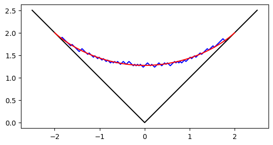
We can display the resulting (scaled) Young diagram.

x_axis = x_axis_func(result_diag[0], result_diag[1]) * (1.0/np.sqrt(SIM_TIME))
height = height_array(result_diag[0], result_diag[1]) * (1.0/np.sqrt(SIM_TIME))

x_sample = np.linspace(-2, 2, 100)
vkls = (2.0/np.pi)*(x_sample*np.arcsin(x_sample/2)+np.sqrt(4-x_sample**2))

plt.axes().set_aspect('equal')
plt.plot(x_axis, height, color="blue")
plt.plot([-2.5, 0, 2.5], [2.5, 0, 2.5], color="black")
plt.plot(x_sample, vkls, color="red")

We can obtain the following image and can compare the scaled profile and the Vershik–Kerov–Logan–Shepp curve.

result

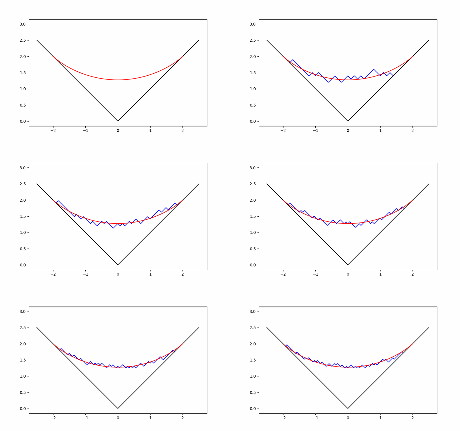
If we want to see an aspects of growth and convergence to the limit shape, we can create a gif image as follows.

fig = plt.figure(figsize=(8, 5))

x_sample = np.linspace(-2, 2, 100)
vkls = (2.0/np.pi)*(x_sample*np.arcsin(x_sample/2)+np.sqrt(4-x_sample**2))

SIM_TIME = 1000
MINS_ORIGIN = np.array([-1, 1])
MAXS_ORIGIN = np.array([0])

diag = (MINS_ORIGIN, MAXS_ORIGIN)

images = []
plt.axes().set_aspect('equal')

for t in range(SIM_TIME):
    x_axis = x_axis_func(diag[0], diag[1])
    height = height_array(diag[0], diag[1])

    x_axis_scal = x_axis*(1.0/np.sqrt(t))
    height_scal = height*(1.0/np.sqrt(t))

    image1 = plt.plot(x_axis_scal, height_scal, color="blue")
    image2 = plt.plot([-2.5, 0, 2.5], [2.5, 0, 2.5], color="black")
    image3 = plt.plot(x_sample, vkls, color="red")
    images.append(image1 + image2 + image3)

    diag = plancherel_growth(diag[0], diag[1])

anime = animation.ArtistAnimation(fig, images, interval=40, blit=True, repeat_delay=0)
anime.save("plancherel_growth.gif", writer="pillow")
plt.show()

We obtain the following gif image.

result